Part 4: compounding returns

As Einstein (maybe) said, compounding interest is the eighth wonder of the world. In the previous posts in this series, we used a very linear benchmark: 4% off of the amount contributed forever. However, this is a weird way to benchmark results. Imagine you and friend (call him Baelish) are both investing and comparing results. You start off by investor $1k in August, 2020 and hope to have $1040 in one year. One year later, you have succeeded and have $1040. You tell your friend Peter Baelish about your investment and he puts $1040 in the market and sets a goal of making 4%: he’ll try to have $1081.60 by next year. However, if you stick with the model used in the previous post, your goal for the year will only be $1080 by 2022, leaving you a whole $1.60 poorer than your friend. (Arguably. We are talking about the benchmark, not the actual amount of money you’re earning. However, this whole series could probably be titled “It’s easy to mislead yourself that you’re doing better than you are,” so it’s fitting the theme)

So instead of a fixed amount, we want to continuous compound our benchmark. Because each value in the benchmark is determined based on the previous one, this is not Pandas-friendly. We’ll have to drop into “normal Python” to compute a more accurate benchmark.

Let’s stick with SPY, making once-a-month $1k contributions with the goal of a 4% annual return. The only difference is that we now want a 4% compounding annual return.

There are 253 trading days in a year and the formula for continuously compounding returns is:

P_t = P₀ * e^rt

That is, the amount you have at time t (P_t) is the amount you have at the beginning of the period (P₀), multiplied by the constant e raised to the rate (4%) times the amount of time. For example, if we contribute $1k and wait 1 year, we’ll want to have:

P₁ = $1000 * e^{4% * 1 year} = $1000 * e^{.04 * 1} = $1040.81

We get an extra $.81 cents off of the continuous compounding.

However, we want to be able to graph this benchmark by the day, so our t isn’t 1, it’s 1 year / 253 days = .00395. Plugging this in, each day we should have e^.00016 more than the previous day. Using the code from previous posts, this gives us:

import math
benchmark = []
idx = 0
for day in df.index:
  contribution = 0
  if day in my_portfolio.index:
    contribution = my_portfolio.loc[day].total_cost_basis
  # The first time through, benchmark is [] (False), so it just adds
  # todays_benchmark. Each subsequent iteration it uses the previous row.
  if benchmark:
    today = benchmark[-1] * math.exp(.004 * (1/253)) + contribution
  else:
    today = contribution
  benchmark.append(today)
df.assign(benchmark=benchmark)[['total', 'benchmark']].plot()

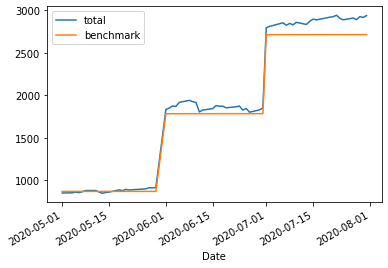
This is, honestly, extremely similar to the original chart. After all, at the end of 1 year we only expect them to have diverged by ~80 cents per $1000! However, over time this number grows, which is clearer if we subtract our cost basis from the benchmark:

(df.assign(cost_basis=my_portfolio.total_cost_basis.cumsum())
    .fillna(method='ffill')
    .assign(performance=lambda x: x.benchmark - x.cost_basis)
    .performance
    .plot())

The nice thing about investing is that your money works “while you sleep” (depending on timezone). Tightening up the benchmark line by using a compounding benchmark lets us hold our money accountable when reviewing performance.